Writing a fourth order Runga Kutta solver for a vibrations problem in Python (Part 1)

Problem

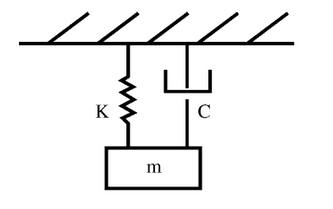
If you want to solve a vibrations problem with a force acting on the system you often need to find the solution in nummerical algorithms. Say you have got a single degree of freedom mass spring system as shown in the figure below.

The differential equation of this system is:

When the force that acts on the system is a function, this problem can be solved with symbolical maths by solving the differential equation. However if raw measured vibration data is used the problem needs to be solved nummerically.

Euler method

Before we can solve the problem mentioned above we are first going to take a look at nummerical methods for first first order ordinary differential equations (ode’s). These are differential equations in the form:

The Runga Kutta method is a nummerical method for solving first order ode’s.

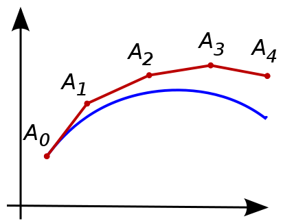
This method determines the tangent line for the derivative of y (y’) for every small step in time dt. So it is possible to describe a yet unknown function by computing the derivative for each small step dt. For this to be possible the start conditions of the curve need to be known. The starting conditions and the derivatives function are the input for this method.

The simplest of the Runga Kutta methods is the Euler method. This method only determines the tangent for each step dt and increments with ti + dt and yt + dy. (dy is the tangent line of y multiplied with dt).

Written in math the Euler method is describes as:

Well I am definitly not a mathmetician, so I understand such methods often a lot better written in code.

def euler(t, f, initial=(0, 0)):
    """
    Eulers nummerical method.

    Computes dy and adds it to previous y-value.
    :param t: (list/ array) Time values of function f.
    :param f: (function) y'.
    :param initial:(tpl) Initial values.
    :return: (list/ array) y values.
    """
    # step size
    h = t[1] - t[0]
    y = np.zeros((t.size, ))

    t[0], y[0] = initial

    for i in range(t.size - 1):
        y[i + 1] = y[i] + h * f(t[i], y[i])

    return y

The first parameter is a numpy array of the time values t. The second parameter is a function that should return y’. In the case of:

the function should return

# Note that the t values is not needed for this problem.
def func(t, y):
    return y

The third parameter tuple are the starting conditions (t0, y0).

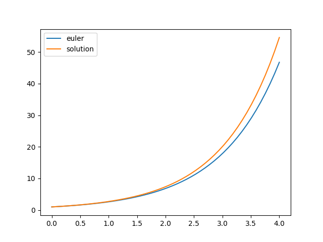
If we compare the output of the Euler method wit the real solution y = exp(t) we see that this nummerical method deviates quite a lot.

import numpy as np
import matplotlib.pyplot as plt

# initiate the time values.
t = np.linspace(0, 4, 50)


def solution(t):
    return np.exp(t)


plt.plot(t, euler(t, func, initial=(0, 1)), label="euler")
plt.plot(t, solution(t), label="solution")
plt.legend()
plt.show()

This deviation from the real solution can be decreased by minimizing the step size, but overall this method should not be used for acquiring accuracy. To get more accuracy we are going to do the same in a 4th order Runga Kutta method in the next post.

READ HERE FOR THE NEXT PART!