Writing a fourth order Runga Kutta solver for a vibrations problem in Python (Part 2)

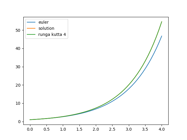
This post continues where part 1 ended. In order to increase the accuracy of our function solver we are going to use a 4th order Runga Kutta algorithm. The basics are the same as with the Euler method. However the dy part of the 4th order method is more accurately computed.

Definition

The incremental values of this method are defined as:

With the factors k₁ - k₄ being:

The function f is again the derivative of y.

Code

Lets see how this looks in Python.

def runga_kutta_4(t, f, initial=(0, 0)):
    """
    Runga Kutta nummerical method.

    Computes dy and adds it to previous y-value.
    :param t: (list/ array) Time values of function f.
    :param f: (function)
    :param initial:(tpl) Initial values
    :return: (list/ array) y values.
    """
    # step size
    h = t[1] - t[0]
    y = np.zeros((t.size, ))

    t[0], y[0] = initial

    for i in range(t.size - 1):
        k1 = h * f(t[i], y[i])
        k2 = h * f(t[i] + h * 0.5, y[i] + 0.5 * k1)
        k3 = h * f(t[i] + h * 0.5, y[i] + 0.5 * k2)
        k4 = h * f(t[i + 1], y[i] + k3)
        y[i + 1] = y[i] + (k1 + 2 * k2 + 2 * k3 + k4) / 6
    return y

As you can see above the input values are the same as with euler function. Again the starting point of the curve must be set by passing the initial values for t₀ and y₀.

By plotting all 3 curves, the Euler method, the 4th order Runga Kutta method and the function y = e^t than we find that the curve of the Runga Kutta method is plotted above the curve of the solution and thus has far more acccuracy than the Euler method.

In the next post we are going to apply the Runga Kutta solution to the vibrations problem.

READ HERE FOR THE NEXT PART!