The Dutch SBR guideline is intended to help you process vibration data and help you determine when a vibration signal can cause discomfort to persons. It seems to me however, that the SBR-B guideline does not have the intention to be understood. They seem to help you by making a super abstract of scientific papers and by giving you a few keywords so you can Google it yourself.
This post will elaborate on two formula’s given in the guideline. It took me a while to find out what they really ment. But thanks to some help from my colleague Lex van der Meer, and some papers he found, I could make sense of it.
Problem
The guideline gives two formula’s that should be used to turn your raw data from a vibrations measurement into design values for further processing. Roughly translated, in about the same amount of words, it says:
The vibration data needs to be weighed by:
In which:
| f | frequency in Hz |
| f0 | 5.6 Hz |
| v0 | 1 mm/s |
From the result of the formula above the effective value is determined by:
In which:
In the first formula a frequeny in Hz is required. They do not specify which frequency. I thought my measured vibration signal had infinity frequencies, or at least more than one? In the second formule we integrate the output of the first formula over dξ, again not specifying what ξ is. That’s about all the attention the guideline spents on it. Well good luck with that!
Time signal
First we need some ‘measured’ data. In the following code snippet some fake data is created by adding 5 sine waves. The sine waves’ amplitudes and frequency are random.
import numpy as np
import matplotlib.pyplot as plt

np.random.seed(5)
t = np.linspace(0, 2.5, 500)
vibrations = np.zeros_like(t)

for i in range(5):
    vibrations += np.sin((10 * np.random.rand())**2 * 2 * np.pi *t) * 10 * np.random.rand()

fig = plt.figure(figsize=(12, 6))
plt.title("Measured vibration")
plt.ylabel("v [mm/s]")
plt.xlabel("t [s]")
plt.plot(t, vibrations)
plt.show()
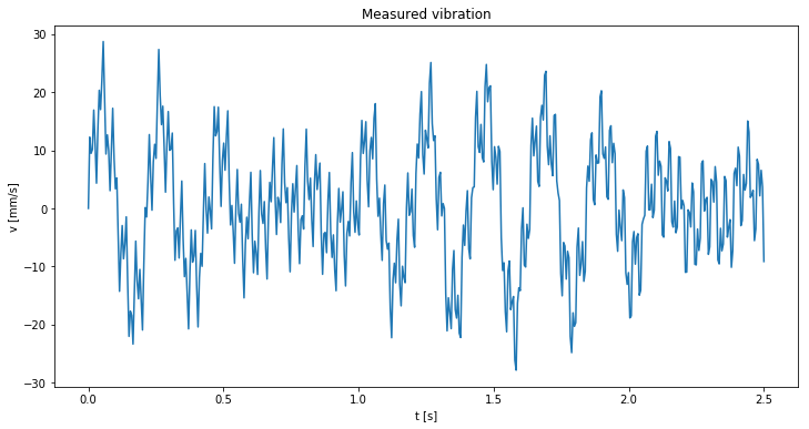
Vibration signal
Above is the fake vibration data we’ve just created shown. Now we have a vibrations signal we can take apart the two give formula’s and see what their use is.
Weighted signal
The first formula is used to weight the signal by the frequencies that are most likely to cause hindrance. This becomes more clear if we plot the function first. Let’s plot the result of the function in the frequency range 1 - 100 Hz. Note that 1 / v0 = 1, thus let’s ignore that.
f = np.arange(0, 100)
f0 = 5.6
y = 1 / np.sqrt(1 + (f0/f)**2)

plt.plot(f, y)
plt.xlabel("f [Hz]")
plt.show()
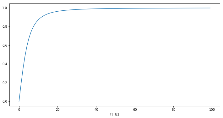
Weight function
By plotting \(\frac{1}{\sqrt{1 + (f/5.6)^2}}\) in the range 1-100 Hz we get the curve shown above. Apparently the lower frequencies will be weighted much more than the higher ones, as the the curve will tend to go to zero by increasing the frequency. This weighting is done by multiplying the original signal with this function.
What the guideline does not mention is that before you are able to do so, you must convert the signal from the time domain to the frequency domain. Well, this can be done by taking the Fast Fourier Transform! You can read more about this in the last post.
By taking the FFT we retrieve the frequency bins. Each bin can be multiplied with the weights function. Shown below is the frequency spectrum and the curve that will scale down this spectrum.
vibrations_fft = np.fft.fft(vibrations)
T = t[1] - t[0]
N = t.size

f = np.linspace(0, 1 / T, N)
a = N // 2

weight = 1 / np.sqrt(1 + (5.6/f)**2)
vibrations_fft_w = weight * vibrations_fft

fig = plt.figure(figsize=(14, 4))
plt.subplot(121)
plt.title("Frequency spectrum")
plt.ylabel("[-]")
plt.xlabel("f [Hz]")
plt.bar(f[:a], np.abs(vibrations_fft[:a]) / np.max(vibrations_fft[:a]), width=0.3)
plt.plot(f[:a], weight[:a], c="r")

plt.subplot(122)
plt.title("Weighted frequency spectrum")
plt.ylabel("[-]")
plt.xlabel("f [Hz]")
plt.bar(f[:a], np.abs(vibrations_fft_w[:a]) / np.max(vibrations_fft[:a]), width=0.3)
plt.ylim(0, 1)
plt.show()
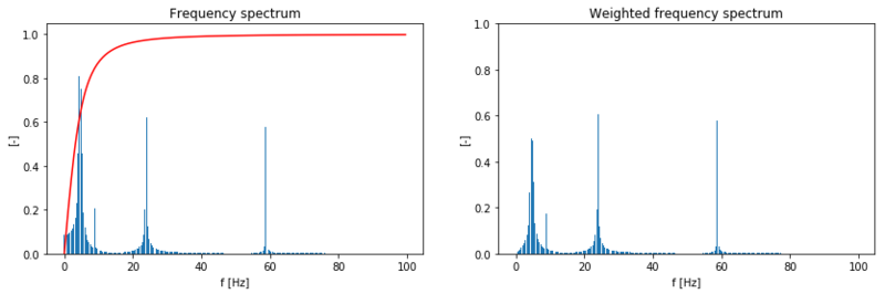
Weighted frequency spectrum
The above figure shows that all frequencies are downscaled. However the lower frequencies are downscaled most. The higher frequencies are probably leading to the most hindrance. And very low frequencies will probably just rock you to sleep.
By transforming the signal back to the time spectrum we can see how the frequency scaling affected the signal.
vibrations_w = np.fft.ifft(vibrations_fft_w).real

plt.title("Weighted vibration")
plt.ylabel("v [mm/s]")
plt.xlabel("t [s]")
plt.plot(t, vibrations_w)
plt.show()
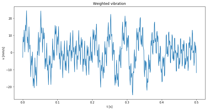
Weighted time spectrum
By comparing the above figure with the original signal we can see it has changed a bit. By weakening the lower frequencies the signal has decreased in amplitude. The maximum amplitude has dropped from ~ 30 mm/s to ~ 25 mm/s.
Effective value
The second formula describes how you can compute the effective value of the vibration signal, or ‘voortschrijdende effectieve waarde’ in Dutch. This formula looks a lot like the formula of the Root Mean Square (RMS) of a signal. The formula of the RMS given by:
It resembles the first formula. However for \(v(t - \xi)\) the velocity signal is multiplied with \(e^{-\xi/\tau}\). Also the signal is not an integral with steps dt, but an integral with steps dξ
The ξ is actually another parameter for the time t. Every increment in time dt a new integral is computed from t0 to ti with steps dξ (which are the same size as dt); The function \(e^{-\xi/\tau}\) is another scaling function. The larger ξ becomes, the smaller the multiplication factor becomes.
v_sqrd_w = vibrations_w**2
a = 55
c = ["#1f77b4" for i in range(a)]

current = 51
c[current] = "#d62728"

xi = t[:current + 2]
g = np.exp(-xi / 0.125)

plt.subplot(211)
plt.title("Squared signal")
plt.plot(t[:current + 2], g[::-1][:a] * v_sqrd_w[current + 1], color="r")
plt.bar(t[1:a], v_sqrd_w[1:a], width=0.002, color=c)
plt.ylim(0, np.max(v_sqrd_w))

for i in range(g.size):
    v_sqrd_w[i] *= g[-i]

plt.subplot(212)
plt.title("Weighted squared signal")
plt.xlabel("t [s]")
plt.bar(t[1:a], v_sqrd_w[1:a], width=0.002, color=c)
plt.ylim(0, np.max(vibrations_w**2))
plt.show()
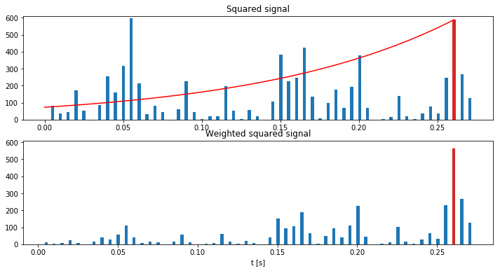
Scaled down time signal per time step
In the code snippet above the signal is squared and plotted. The red bar in the plot is the current time inteval ti. All the preceding values of, and including the value for v(t)2, will be multiplied with the red function. This function ranges from 0 to 1. Values close to the current time interval ti will keep their value. Values further away will be scaled down more. This multiplication is done for every time step ti. The scaled down signal for the current time step is shown the in the second figure.
When the weighted value for every time step is determined the RMS can be computed for this weighted signal.
Ts = 0.125
v_eff = np.zeros(t.size)
dt = t[1] - t[0]

for i in range(t.size - 1):
    g_xi = np.exp(-t[:i + 1][::-1] / Ts)
    v_eff[i] = np.sqrt(1 / Ts * np.trapz(g_xi * v_sqrd_w[:i + 1], dx=dt))

plt.plot(t, v_eff)
plt.title("Effective value")
plt.ylabel("v [mm/s]")
plt.xlabel("t [s]")
plt.show()
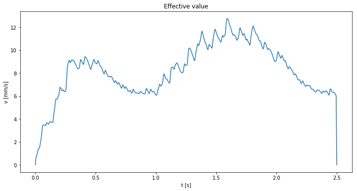
Effective value time signal
Conclusion
We have computed the effective value (voortscrhijdende effectieve waarde) for a random time signal. It was quite a hassle for me to find out what should be done. The guideline does not mention that you need to switch between the frequency and the time spectrum two times. Also the interpretation of ξ in the second formula could really use a calculation example.
What you eventually can do with the computed effective value is something I will leave to the guideline. I hope this helps someone a few hours when dealing with the SBR!