Recap
Last post I described what my motivations were to start building a music classifier, or at least attempt to build one. The post also described how I collected a dataset, extracted important features and clustered the data based on their variance. You can read the previous post here.
This post describes how I got my feet wet with classifying music. Spotify kind of sorted the data I’ve downloaded by genre. However when I started looking at the data, I found that a lot of songs were interchangeable between the genres. If I am to use data that do not belong solely to one class but should be labeled as both soul and blues music, how can a neural network learn to distinguish between them?
Take the genres blues and rock as an example. In the data set both genres contained the song Ironic made by Alanis Morissette. In my opinion this songs doesn’t belong to any of these genres. To address this problem I chose to train the models on the more distinguishable genres, namely:
| Genre | No. of songs |
|---|---|
| Hiphop | 1212 |
| EDM | 2496 |
| Classical music | 2678 |
| Metal | 1551 |
| Jazz | 417 |
I believe that these genres don’t overlap too much. For instance a metal song can have multiple labels, but I am pretty sure classical and jazz won’t be one.
Now the genres are chosen, the data set is still far from perfect. As you can see in the table above the data is not evenly distributed. So I expect that the trained models will find it harder to generalise for music that is less represented in the data. Jazz music for instance will be harder to train than classical music as the latter is is abundant in the data set.
Another example of the flaws in the data set is that there are songs that aren’t even songs at all! During training I realised that the data set contained songs that were labeled as metal. When actually listening to the audio they seemed to be just recordings of interviews with the band members of Metallica. I really didn’t feel like manually checking every song for the correct label, thus I’ve accepted that the models will learn some flawed data. This luckely gives me an excuse when some predictions are really off :).
Multilayer perceptron
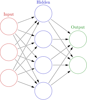
The first models I trained were multilayer perceptrons also called feed forward neural networks. These nets consist of an input layer, one or multiple hidden layers and an output layer. The output layer should have as many nodes as classes you want to predict. In our case this would be five nodes. The figure below shows an example of a multilayer perceptron.
Multilayer perceptron
data augmentation
In the last post I described that the feature extraction has converted the raw audio data into images. Every pixel of these images is an input to the neural network. As we can see in the figure above. Every input is connected to all the nodes of the next layer. Lets compute the number of parameters this would take for a neural net with one hidden layer for one song’s image.
As a rule of thumb we can choose the number of hidden nodes somewhere between the input nodes and the output nodes.
The input image has a size of \(10 x 2548 = 25,480 \) pixels. The number of output nodes is equal to the number of classes = 5 nodes. If we interpolate the amount of hidden layer connections:
The total connections of the neural net would become:
This sheer number of connections for a simple neural net with one hidden layer was way too much for my humble laptop to deal with. Therefore I started to reduce the amount of input data.
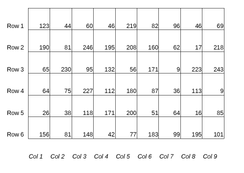
Computers see images as 2D arrays of numbers. Below is an example shown of a random grayscale image of 9x6 pixels. The pictures I used to classify information contain MFCC spectra. Every column of these images is a discrete time step ti and contains time information. The rows contain frequency coefficient information.
Grayscale picture (as a computer sees it)
I reduced the amount of information by only feeding every 20th column of the image. This way the frequency information of a timestep ti remains intact however the amount of time steps is divided by 20. This is of course a huge loss of information, but the upside of this rough downsampling was that I could expand my data set with 20 times the amount of data. As I could just change the offset of counting every 20th column. The amount of input nodes reduced to \(\frac{25480}{20} = 1274 \) nodes. Which is a number of input nodes my laptop can handle and gives me the possibility expand the network deeper.
model results
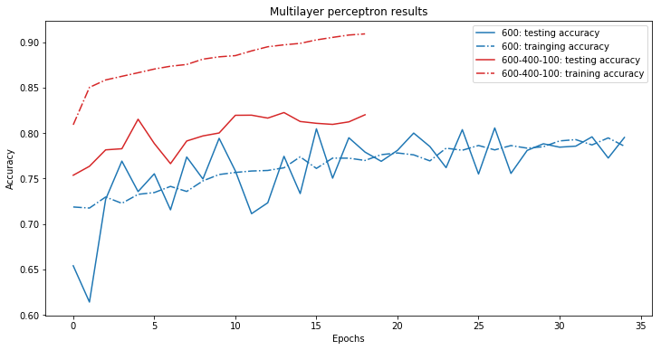
The best results were yielded from a model with one hidden layer and a model with three hidden layers. The amount of hidden nodes were divided as following:
- Model 1; hidden layer 1; 600 nodes
- Model 2; hidden layer 1; 600 nodes
- Model 2; hidden layer 2; 400 nodes
- Model 2; hidden layer 1; 100 nodes
To prevent the models from overfitting I used both l2 regularisation and dropout. 20% of the total data set was set aside as validation data.
Below are the results plotted. The dashed lines show the result the accuracy of the models on the training data. The solid lines are the validation data results. This is an indication of how accurate the models are on real world data. As in music they haven’t heard before, or in this case music they haven’t seen before.
Accuracy of the feed forward models
The maximum accuracy on the validation set was 82%. I am quite pleased with this result as I threw away a lot of information with the rigorous dropping of the columns. In a next model I wanted to be able to feed all the information stored in a song’s image to the model. Furthermore it would also be nice if the model could learn something about the order of frequencies. In other words that the model learns something about time information, maybe we can even call it rhythm.
I don’t believe a feed forward neural net does this. For a feed forward network I need the rescale the 2D image matrix into a 1D vector which probably is also some (spatial) information loss.
Convolutional
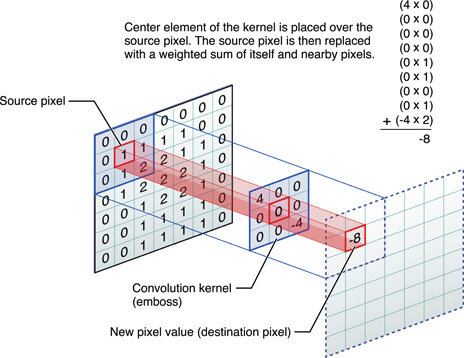
I believe the solution to some of the wishes I named in the last section are convolutional neural networks (CNN). Convolutional neural networks work great with images as they can deal with spatial information. An image contains 2D information. The input nodes of a CNN are not fully connected to every layer so the model can deal with large input data without blowing up the amount of nodes required in the model. Images can have a high number of megapixels, thus a lot of data. I think these properties of CNN are also convenient for our problem of classifying music images.
Convolutional neural network in action
shared nodes
In a convolutional neural net the weights and biases are shared instead of fully connected to the layers. For an image this means that a cat in the left corner of an image leads to the same output as the same cat in the right corner of an image. For a song this may be that a certain rythm at the beginning of song will fire the same neurons as that particular rhythm at the end of the song.
spatial information
The images I have created in previous post contain spatial information. As said before the x direction shows time information, the y directions shows frequency coefficients. With CNN’s I don’t have to reshape the image matrix in a 1D vector. The spatial information stays preserved.
data set
Both the shared nodes and the spatial information preservation does intuitively seem to make sense. The only drawback compared to the previous model is the amount of data. By the drastic downsampling in columns I was able to created a twentyfold of the original number of songs. Now I was feeding the whole image to the model. So the amount of data remains equal to the amount of downloaded songs.
In image classification the data sets are often augmented by rotating and flipping the images horizontally. This augmentation seems reasonable as a rotated cat is still a cat. The proof of this statement is provided! I am not certain this same logic is true for music. Doesn’t a rotated songs image hustle some time and frequency information? I am not sure about the previous statement, thus I chose to leave the songs images intact and work with the amount of songs I’ve got.
results
The convolutional models yielded far better results than the feed forward neural nets. The best predicting model contained 3 convolutional layers with respectively 16, 32 and 32 filters. After the convolutional layers there was added a 50% dropout layer followed by a fully connected layer of 250 neurons. For who is interested in all the technicalities a graph of the model is available here.
The accuracy gained during training of the two best predicting models are shown in the plot below.
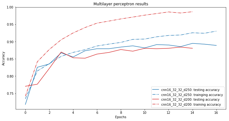
Accuracy of the convolutional neural nets
The nummerical results in terms of the prediction accuracy are shown in the table below. Note that the accuracy results was computed with all the data, training and validation data. On real world data the results would probably be a bit lower.
| precision | recall | n songs | |
|---|---|---|---|
| Hiphop | 0.87 | 0.94 | 1208 |
| EDM | 0.95 | 0.91 | 2493 |
| Classical | 0.97 | 0.98 | 2678 |
| Metal | 0.96 | 0.97 | 1571 |
| Jazz | 0.86 | 0.78 | 416 |
The table shows the precision and the recall of the labels. The precision is the amount of good classifications divided by the total amount times that label was predicted. Recall is the amount of good classifications divided by the total occurrences of that specific label in a data set. So let’s say I’ve trained my model very badly and it only is able to predict jazz as a label. Such a hypothetical model would have 100% recall on the jazz label.
- Total number of songs: 11,366
- Total number of jazz songs: 416
The precision of the model would however be low as the model has classified all the songs as jazz.
So back to the table we can see that EDM, metal and classical music score best on both precision and recall. Hiphop has a good recall score. It scores a bit lower on precision meaning that it mostly correct in labeling a hiphop song given that it is a hiphop song, but the model makes more mistakes by labeling a song as hiphop that should not be classified as such. Jazz scores worst. Which is as expected as the amount of jazz songs in the data set is substantially lower than the other labels.
tl;dr
This post focusses on the classification of the songs. I’ve described the results I yielded with feed forward and convolutional neural networks that classified music based on MFCC images.
The convolutional model is used in the small widget below. You can try to search by an artist and a track name. If a match is found in the spotify library an mp3 is downloaded and converted to a MFCC image. When the model has finished ‘viewing’ the song it will make his best prediction of the known labels.
Before a prediction can be made the mp3 needs to be downloaded, converted to a .wav audio file, converted to a MFFC image and finally fed to the model. I only have got a small web server, so please be patient. A prediction is coming your way. :)
Oh and remember… it only knows:
- Hiphop
- EDM
- Classical music
- Metal
- Jazz
It is of course also interesting to see how the model classifies genres it hasn’t learned. But I cannot promise you it would be a sane prediction though.
Update 11-04-2019
The widget below doesn’t work because I didn’t want to maintain the backend anymore.