Intro
At the moment of writing this post it has been a few months since I’ve lost myself in the concept of machine learning. I have been using packages like TensorFlow, Keras and Scikit-learn to build a high conceptual understanding of the subject. I did understand intuitively what the backpropagation algorithm and the idea of minimizing costs does, but I hadn’t programmed it myself. Tensorflow is regarded as quite a low level machine learning package, but it still abstracts the backpropagation algorithm for you. In order to better understand the underlying concepts I’ve decided to build a simple neural network without any machine learning framework. In this post I describe my implementation of a various depth multi layer perceptron in Python. We’ll be only using the Numpy package for the linear algebra abstraction.
1. Network
This part of the post is going to walk through the basic mathematical concepts of what a neural network does. In the same time we are going to write the code needed to implement these concepts.
We are going to build a three layer neural network. Figure 1 shows an example of a three layered neural network. This is the minimum required amount of layers when talking of a multi layer perceptron network. Every neural net requires an input layer and an output layer. The remaining layers are the so called hidden layers. The input layers will have data as input and the output layers will make predictions. Such a prediction can be a continuous value like stock market prices or could be a label classifying images.
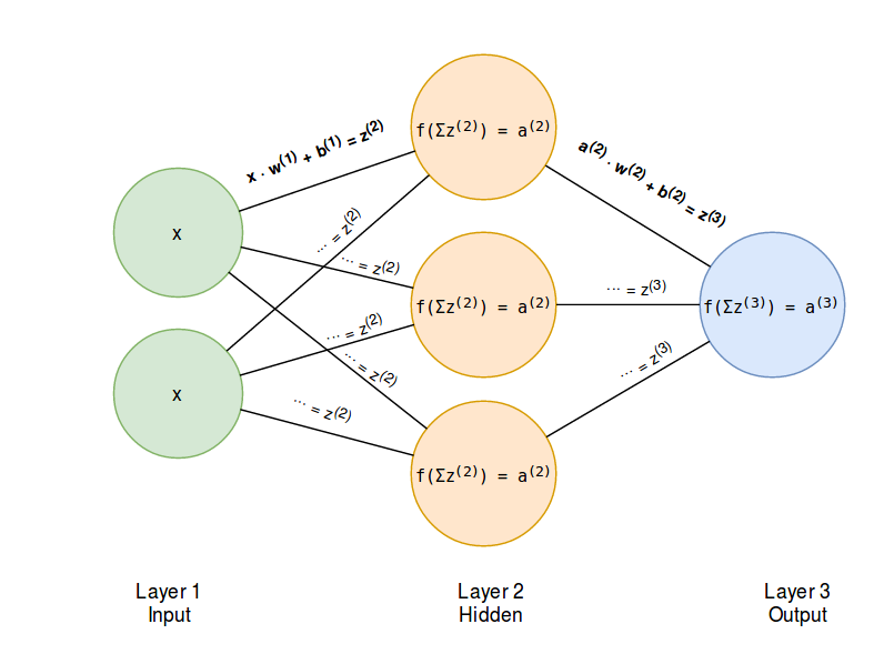
Image 1: Feed forward pass of a neural network
1.1 Single layer
The mathematics of a single layer are the same for every layer. This means that we can focus on the mathematical operations of a single layer and later apply it to the whole network. We are now looking at the first layer of the network.
If we look at this first layer, it has got a certain input vector \( \vec{x} \) representing the data. This data is multiplied with the weights \( \vec{w} \) and shifted over \( \vec{b} \). The output is:
Note that \( \odot \) means the Hadamard product and is just elementwise multiplication. If we would make this visual in vector or neuron form it would look something like this.
Vector form
Neuron form
The figures above show the connection of three input nodes to one node of a hidden layer. The output vector is eventually summed resulting in one scalar output in the hidden layer node. The output of a hidden layer node is the input for the next layer. As you can see the process repeats until the neural networks generates an output.
Note that we can also replace the bias vector with one bias scalar. By doing so we can use the dot product of the weights and the activations of the previous layer \( x \).
1.2 Non linearity
As discussed above figure 1 shows a network that consists of inputs. The input vector \( \vec{x}\) is multiplied with \( \vec{w} \) and shifted along \( \vec{b} \), the weights and biases of the first layer. The second layer seems to repeat the same math operation, only with other weights and biases. This is a concatenation of two linear functions. \( w \cdot x + b \) is a linear function, and feeding the output of \( w^{(1)} \cdot x + b^{(1)} \) in \( w^{(2)} \cdot x + b^{(2)} \) will result in another linear function. If we assume that our network is properly trained, we can conclude that the last layer is redundant as the first layer could have already represented the linear function we are looking for.
A concatenation of multiple linear functions can thus be replaced by one linear function and isn’t beneficial to the model. To give the second layer any purpose the output of the first layer \( z \) is multiplied with a non linear function \( f(x) \) resulting in:
The final output a(2) is called the activation of the neuron. In this case we use the supercript 2, as it is the activation of the node in the second layer.
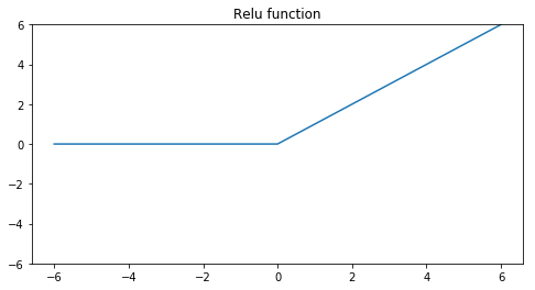
The non linear functions we are going to use are the Relu function and the Sigmoid function.
Relu function:
Sigmoid function:
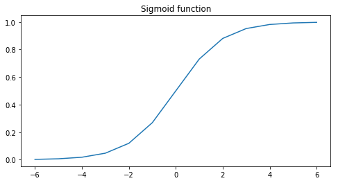
These non linear functions give the network the ability to learn non linear relations in the data and make it possible to learn in more depths of abstraction. The relu function will let every positive value pass through the network. Negative values will be changed to zero so the neuron doesn’t activate at all. The sigmoid function squashes the outputs to a value between zero and one. We can think of this as probabilities. We will use the relu function at the hidden layer and the sigmoid function at the output layer.
1.3 Code
Now that we have got some sort of high level view on what is happening in the net, we can write some code. Just a few variable notations up front:
- w: weights
- b: biases
- z: output of a neuron: \(x \cdot w + b\)
- a: activations of z: \(f(z)\)
Activation functions
First we write the two activation functions. The @staticmethod decorator makes it possible to call the two methods directly from class level so we don’t have to create any objects from the two classes.
import numpy as np


class Relu:
    @staticmethod
    def activation(z):
        z[z < 0] = 0
        return z


class Sigmoid:
    @staticmethod
    def activation(z):
        return 1 / (1 + np.exp(-z))
Network class
Next is the container that will keep the hidden state and perform all the logic for the neural network: the Network class.
class Network:
    def __init__(self, dimensions, activations):
        """
        :param dimensions: (tpl/ list) Dimensions of the neural net. (input, hidden layer, output)
        :param activations: (tpl/ list) Activations functions.

        """

        self.n_layers = len(dimensions)
        self.loss = None
        self.learning_rate = None

        # Weights and biases are initiated by index. For a one hidden layer net you will have a w[1] and w[2]
        self.w = {}
        self.b = {}

        # Activations are also initiated by index. For the example we will have activations[2] and activations[3]
        self.activations = {}

        for i in range(len(dimensions) - 1):
            self.w[i + 1] = np.random.randn(dimensions[i], dimensions[i + 1]) / np.sqrt(dimensions[i])
            self.b[i + 1] = np.zeros(dimensions[i + 1])
            self.activations[i + 2] = activations[i]
In the __init__ function we initiate the neural network. The dimensions argument should be an iterable with the dimensions of the layers. Or in other words the amount of nodes per layer. The activations argument should be an iterable containing the activation class objects we want to use. We need to create some inner state of weights and biases. This inner state is represented with two dictionaries self.w and self.b. In the for loop we assign the chosen dimensions to the layer numbers. A neural network containing 3 layers; input layer, hidden layer, output layer will have weights and biases assigned in layer 1 and layer 2. Layer 3 will be the output neuron.
We can see that the biases are initiated as zero and the weights are drawn from a random distribution. The dimensions of the weights are determined by the dimensions of the layers. The drawn weights are eventually divided by the square root of the current layers dimensions. This is called Xavier initialization and helps prevent neuron activations from being too large or too small.
So if we want to initiate a neural network with the same dimensons as the one in figure 1 we could create an object from the Network class. I’ve set the random seed to 1 in order to reproduce the same outputs.
initialization
np.random.seed(1)
nn = Network((2, 3, 1), (Relu, Sigmoid))
If we print the weights and biases we will receive the following dictionaries. As said in the first part of the post, every input neuron is connected to all the neurons of the next layer, resulting in 2 * 3 = 6 weights in the first layer and resulting in 3 * 1 = 3 weights in de second layer. Because we’ve chosen to add the biases after the summation has taken place, we only need as many biases as there are nodes in the next layer.
The following snippet shows the location of the internal state of the network. The keys represent the layers, the values represent the weights, biases and activation classes.
internal state
Weights:
{
	1: array([[ 1.14858562, -0.43257711, -0.37347383],
	       [-0.75870339,  0.6119356 , -1.62743362]]),
	2: array([[ 1.00736754],
	       [-0.43948301],
	       [ 0.18419731]])}
}

Biases:
{
	1: array([ 0.,  0.,  0.]),
	2: array([ 0.])
}

Activation classes:
{
	2: <class '__main__.Relu'>,
	3: <class '__main__.Sigmoid'>
}
1.3 Feeding forward
Now we are going to implement the forward pass. The forward pass is how the network generates output. The inputs that are fed into the network are multiplied with the weights and shifted along the biases of every layer (if they pass through the Relu function) and finaly they pass the sigmoid function resulting in an output between 0 and 1. The mathematics of the forward pass are the same for every layer. The only variable is the activation function \( f(x) \).
However algorithmicly we have abstracted the activation function with activation classes. All the activation classes have got the method .activation(). This means that we can loop over all the layers doing the same mathematical operation. Finally we call the varying activation function with the .activation() method. We add a ._feed_forward() method to the Network class.
    def _feed_forward(self, x):
        """
        Execute a forward feed through the network.

        :param x: (array) Batch of input data vectors.
        :return: (tpl) Node outputs and activations per layer.
                 The numbering of the output is equivalent to the layer numbers.
        """

        # w(x) + b
        z = {}

        # activations: f(z)
        a = {1: x}  # First layer has no activations as input. The input x is the input.

        for i in range(1, self.n_layers):
            # current layer = i
            # activation layer = i + 1
            z[i + 1] = np.dot(a[i], self.w[i]) + self.b[i]
            a[i + 1] = self.activations[i + 1].activation(z[i + 1])

        return z, a
We create two new dictionaries in the function z and a. In these dictionaries we append the outputs of every layer, thus again the keys of the dictionaries map to the layers of the neural network. Note that the first layer has no ‘real’ activations as it is the input layer. Here we consider the inputs x as the activations of the previous layer.
The dictionaries structure looks like this.
a:
{
	1: "inputs x",
	2: "activations of relu function in the hidden layer",
	3: "activations of the sigmoid function in the output layer"
}

z:
{
	2: "z values of the hidden layer",
	3: "z values of the output layer"
}
The last thing we need is a .predict() method.
    def predict(self, x):
        """
        :param x: (array) Containing parameters
        :return: (array) A 2D array of shape (n_cases, n_classes).
        """
        _, a = self._feed_forward(x)
        return a[self.n_layers]
2. Learning
Well, that’s nice. We now have created a neural network that can produce outputs based on inputs. However the neural network in this state is still quite useless. Slightly understating, the chance of us initializing the weights and biases just right are pretty slim. In this part we are going through the math and the code required to make the network learn. This part is going to be quite mathematical, but it shouldn’t be too hard, as it is most repetition of the same concept. It will help if you keep an eye on the superscript notations. These notations will tell you in which layer we are in the network.
2.1 Loss function
The network should be able to learn and optimize its inner state. This is done by minimizing a loss function. A loss function describes the rate of error of the predictive power of a neural network. We define a loss function that gives high error rates when the model is very bad at predictions and low error rates when the model gives good predictions. The loss function we define is dependent of the weights and biases of the model. We can tweak the weights and the biases in such a way the output of loss function declines, minimizing the loss function and maximizing the predictive power of the neural network. As a lost function (J) we use the squared error loss.
Where \( y \) is the neural networks prediction and \( \hat{y} \) is the ground truth label, the real world observation.
Gradient descent
Ok, now let’s think about this intuitively. The loss function gives us information about the prediction error of the model. Our goal is to minimize the output of the loss function by minimizing the weights and biases. We know from calculus that if we take the partial derivative of the loss function with respect to a certain weight \( w_i \) we get the gradient of the curve \( \frac{\partial{J}}{\partial{w_i}} \) in that direction. In other words we get information of how much the weight \( w_i \) contributes to the loss functions output. The opposite direction of \( \frac{\partial{J}}{\partial{w_i}} \) points to the direction that minimizes the output of the loss function.
We can go in this opposite direction by reducing the value \( w_i \) with a fraction of \( \frac{\partial{J}}{\partial{w_i}} \). By doing so we reduce the loss functions error and we get a slightly better prediction in the future. This weight optimization is called gradient descent and is done with every weight and bias of the network.
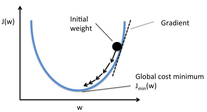
Image 2: Minimize the loss function J(w) by updating the weights.
Chain rule
To determine the partial derivative of J with respect to a certain weight, we need to apply the chain rule in differentiation, meaning we can break the problem down in subsequent multiplications of derivatives. The chain rule is noted as:
And because of the sum rule in differentiation we can also say that the derivative of the sum is equal to the sum of the derivates, therefore we can lose the sum sign in the loss function and determine the derivative of a single weight.
In the following part we are going to walk through the derivation of the partial derivatives of a single weight in layer one and a single weight in layer two. In reality we are going to apply this to a whole batch of weights, but for now we’ll just consider one. Figure 3 shows the notations we’ll use. Note that the derivation of the partial derivatives follows the direction of the green arrow. We are going to backpropagate the error up until the weight we are considering.
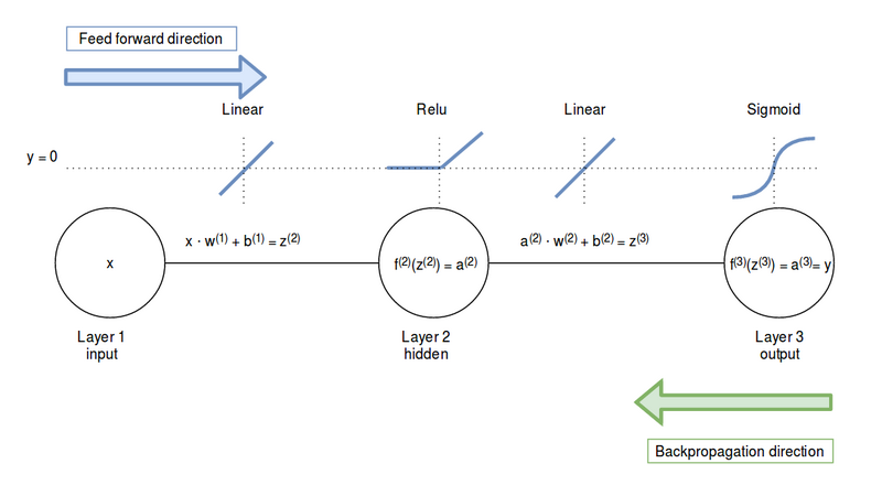
Image 3: Notation of the functions in the three layer network.
2.2 Weights layer 2
So let’s start with the derivative of a weight in layer 2, \( w^{(2)} \). If we apply the chain rule upon \( w^{(2)} \), we derive:
We are grouping the first two derivatives of the formula above in a new variable \( \delta^{(L)} \) where the superscript L means ‘Last layer’.
Breaking apart the two derivates that make up \( \delta^{(L)} \) we find:
- \( \frac{\partial{J}}{\partial{y}} \): Derivate of the loss function with respect to the prediction y.
- \( \frac{\partial{y}}{\partial{z^{(3)}}} \): Derivate of the sigmoid function with respect to the neurons output z.
Derivative of the loss function
Derivative of the sigmoid function
Coding up
We now have enough mathematical background to write the code for determining \( \delta^{(L)} \). First we need to update our Sigmoid class, so we can call the derivative of the function via the .prime() method.
class Sigmoid:
    @staticmethod
    def activation(z):
        return 1 / (1 + np.exp(-z))

    @staticmethod
    def prime(z):
        return Sigmoid.activation(z) * (1 - Sigmoid.activation(z))
We also need a container for our squared error loss. I’ve chosen to make a class from which we initialize objects by passing the activation function of our last layer in the network. In this case we initialize it with the Sigmoid class. If you like to use another function in the final layer, you can choose to do differently. The MSE class below is able to compute the \( \delta^{(L)} \) via calling the .delta() method. We are going to use this class later on in the network.
class MSE:
    def __init__(self, activation_fn):
        """
        :param activation_fn: Class object of the activation function.
        """
        self.activation_fn = activation_fn

    def activation(self, z):
        return self.activation_fn.activation(z)

    @staticmethod
    def loss(y_true, y_pred):
        """
        :param y_true: (array) One hot encoded truth vector.
        :param y_pred: (array) Prediction vector
        :return: (flt)
        """
        return np.mean((y_pred - y_true)**2)

    @staticmethod
    def prime(y_true, y_pred):
        return y_pred - y_true

    def delta(self, y_true, y_pred):
        """
        Back propagation error delta
        :return: (array)
        """
        return self.prime(y_true, y_pred) * self.activation_fn.prime(y_pred)
Derivative of the z function
The last derivative we need is \( \frac{\partial{z^{(3)}}}{\partial{w^{(2)}}} \). The derivative of the output of
Conclusion weights layer 2
Summing it all up we can conclude that we can define the partial derivative of the loss function with respect to \( w^{(2)} \) as the product of the \( \delta^{(L)} \) and the activations of the layer before the weights (i - 1).
2.3 Weights layer 1
For the weights in the first layer we can start with the chain rule right where we left off with \( \delta^{(L)} \).
Derivative of the z function
For the derivate of \( z^{(3)} \) with respect to the activations of the second layer we find:
Derivative of the activation function
And for the derivate of \( a^{(2)} \) we need to determine the prime of the Relu function:
This derivative is zero for any negative value and one for any positive value.
For simplicity we’ll just note this as:
Resulting in \( \delta^{(2)} \) being:
By substituting eq. (2.3.7) in eq. (2.3.0) we’ll find:
In the equation above we only need to solve the last term.
Conclusion weights layer 1
Just as we did for the weights in layer 2 we can define the partial derivative of the loss function with respect to \( w^{(1)} \) as the product of a backpropagating error \( \delta \) and the activations of the layer before the weights (i - 1).
2.4 Backpropagation formulas single weight
We have derived how we can determine the partial derivates of a single weight. These partial derivates show the direction in which the error function is increasing due to that weight, thus by multiplying the weight in the opposite direction we decrease the error function and have got a learning algorithm!
The important formulas for backpropagation are:
output layer
hidden layers
all layers
updating weights and biases
2.5 Multiple weights and batched inputs
To keep things simple, we have only regarded a single weight in the derivation above. In practice we are going to determine the derivates of all weights at once. We are also going to batch our training data by doing a feedforward pass to determine the loss function and then doing a backpropagation pass to update the weights and biases. This is called stochastic gradient descent, as we randomly choose the batches. This blog post gives you a really nice 3D-view of what minimizing a cost function with stochastic gradienct descent means.
Let’s see how the backpropagation formulas look in vector notation if we used a batch of three inputs. In the following vectors every row is a new training sample.
The notation for a single weight was:
If we rewrite \( f’^{(3)}(z^{(3)}) \) in a shorter notation \( f’ \), the vector notation of the eq. (2.5.0) becomes:
\begin{bmatrix} f’_1 \ f’_2 \ f’_3 \end{bmatrix} =
\begin{bmatrix} \delta_1 \ \delta_2 \ \delta_3 \end{bmatrix} \tag{2.5.1} $$
The next step is multiplying the backpropagating error \( \delta \) with our activities \( a^{(2)}\). For a single weight the notation was:
We have got three nodes in layer 2 and three batched inputs. So our activity matrix has a shape of 3x3. Where every row represents the three nodes per input x.
If we transpose matrix \( a^{(2)}\) and matrix multiply with \( \delta^{(L)} \) we retrieve 3x1 vector representing the three derivatives for our three weights \( w^{(2)} \).
\begin{bmatrix} a^{(2)}{11} \cdot \delta_1 + a^{(2)}{21} \cdot \delta_2 + a^{(2)}{31} \cdot \delta_3 \ a^{(2)}{12} \cdot \delta_1 + a^{(2)}{22} \cdot \delta_2 + a^{(2)}{32} \cdot \delta_3 \ a^{(2)}{13} \cdot \delta_1 + a^{(2)}{23} \cdot \delta_2 + a^{(2)}_{33} \cdot \delta_3 & \end{bmatrix} \tag{2.5.5} $$
These matrix multiplications are way faster in an algorithm than a loop could be, so this is what we are going to implement for our neural net class. The backpropagation formula can be rewritten as:
2.6 Backpropagation method
Ok this was the lengthy math part. I promise nothing but code up ahead. Now we know how we can compute the partial derivatives, we can finally implement the backpropagation algorithm. First we start with an ._update_w_b() method to update the weights and biases of any given layer. The self.learning_rate attribute will control the learning process. The index parameter refers to the layer we want to update and the parameters dw and delta are the partial derivative and the backpropagating error.
    def _update_w_b(self, index, dw, delta):
        """
        Update weights and biases.

        :param index: (int) Number of the layer
        :param dw: (array) Partial derivatives
        :param delta: (array) Delta error.
        """

        self.w[index] -= self.learning_rate * dw
        self.b[index] -= self.learning_rate * np.mean(delta, 0)
Now we can finally implement the backpropagation method ._back_prop(). The inputs are two dictionaries containing the keys with the layer numbers and values representing the results of \( w^{(i)} + b^{(i)} = z^{(i)} \) and the activations \( a^{(i)} \). The derivative dw and delta of the last layer are determined outside the for loop, as they differ from the other layers. Next we determine dw and delta for the remaining layers inside the for loop. Because the backpropagation is in the opposite direction, we reverse the loop, starting at the last layer.
dw and delta are added to a dictionary update_params where the keys represent the layer numbers and the values are a tuple containing (dw, delta). When all derivatives of all the layers are determined, a second for loop runs to update our weights and biases.
    def _back_prop(self, z, a, y_true):
        """
        The input dicts keys represent the layers of the net.

        a = { 1: x,
              2: f(w1(x) + b1)
              3: f(w2(a2) + b2)
              }

        :param z: (dict) w(x) + b
        :param a: (dict) f(z)
        :param y_true: (array) One hot encoded truth vector.
        """

        # Determine partial derivative and delta for the output layer.
        # delta output layer
        delta = self.loss.delta(y_true, a[self.n_layers])
        dw = np.dot(a[self.n_layers - 1].T, delta)

        update_params = {
            self.n_layers - 1: (dw, delta)
        }

        # In case of three layer net will iterate over i = 2 and i = 1
        # Determine partial derivative and delta for the rest of the layers.
        # Each iteration requires the delta from the previous layer, propagating backwards.
        for i in reversed(range(2, self.n_layers)):
            delta = np.dot(delta, self.w[i].T) * self.activations[i].prime(z[i])
            dw = np.dot(a[i - 1].T, delta)
            update_params[i - 1] = (dw, delta)

	# Update the weights and biases
        for k, v in update_params.items():
            self._update_w_b(k, v[0], v[1])
2.7 Tying it all together
There is only one method left for a working neural network. The .fit() method will implement the control flow of the training procedure. It will start an outer loop running n epochs. Every new epoch the training data will be shuffled. The inner loop will go through the training data in step sizes of the batch_size parameter. The inner loop computes the \( \vec{z} \) and \( \vec{a} \) vector in the forward pass and feeds those in the ._back_prop() method applying backpropagation on the internal state.
    def fit(self, x, y_true, loss, epochs, batch_size, learning_rate=1e-3):
        """
        :param x: (array) Containing parameters
        :param y_true: (array) Containing one hot encoded labels.
        :param loss: Loss class (MSE, CrossEntropy etc.)
        :param epochs: (int) Number of epochs.
        :param batch_size: (int)
        :param learning_rate: (flt)
        """
        if not x.shape[0] == y_true.shape[0]:
            raise ValueError("Length of x and y arrays don't match")
        # Initiate the loss object with the final activation function
        self.loss = loss(self.activations[self.n_layers])
        self.learning_rate = learning_rate

        for i in range(epochs):
            # Shuffle the data
            seed = np.arange(x.shape[0])
            np.random.shuffle(seed)
            x_ = x[seed]
            y_ = y_true[seed]

            for j in range(x.shape[0] // batch_size):
                k = j * batch_size
                l = (j + 1) * batch_size
                z, a = self._feed_forward(x_[k:l])
                self._back_prop(z, a, y_[k:l])

            if (i + 1) % 10 == 0:
                _, a = self._feed_forward(x)
                print("Loss:", self.loss.loss(y_true, a[self.n_layers]))
3. Validation
That was all the code needed for implementing a vanilla multi layer perceptron. There is only one thing left to do, and that is validation of the code. We need to make sure the algorithm is indeed learning and isn’t just a pseudo random number generator.
As validation the small script below imports a dataset from the sklearn package. The dataset contains flattened images of the digits 1-9. By flattened we mean the 2D matrix containing the image’s pixels is reshaped to a 1D vector. The y variable contains the labels of the dataset, being numbers from 1-9. The labels are stored as ‘one hot encoded’ vectors. This Quora question has a good answer to why we use one hot encoding!
from sklearn import datasets
import sklearn.metrics
np.random.seed(1)
data = datasets.load_digits()

x = data["data"]
y = data["target"]
y = np.eye(10)[y]

nn = Network((64, 15, 10), (Relu, Sigmoid))
nn.fit(x, y, loss=MSE, epochs=100, batch_size=15, learning_rate=1e-3)

prediction = nn.predict(x)

y_true = []
y_pred = []
for i in range(len(y)):
y_pred.append(np.argmax(prediction[i]))
y_true.append(np.argmax(y[i]))

print(sklearn.metrics.classification_report(y_true, y_pred))
Next we create an object nn from the Network class. The size of the first layer and the last layer are defined by our problem. The images have got 64 pixels, thus we need 64 input nodes. There is a total of 10 digits, resulting in 10 output nodes. The size of the hidden layer is arbitrary chosen to be 15.
The nn.predict() method returns probabilities for every digit. We append the maximum argument (being the highest prediction) to a y_true and y_pred variable, representing the ground truth labels and the neural nets prediction respectively.
Finally we print a classification report to see how well the neural net has performed for every single digit. The output is shown below.
             precision    recall  f1-score   support

          0       1.00      1.00      1.00       178
          1       0.99      1.00      1.00       182
          2       1.00      1.00      1.00       177
          3       0.99      1.00      1.00       183
          4       1.00      1.00      1.00       181
          5       1.00      0.99      1.00       182
          6       1.00      1.00      1.00       181
          7       1.00      1.00      1.00       179
          8       1.00      0.99      1.00       174
          9       0.99      0.99      0.99       180

avg / total       1.00      1.00      1.00      1797
After 100 epochs the neural net is able to almost classify all the digits in the dataset and thus is learning!
That is all the mathematics and code needed for the implementation of a multi layer perceptron. This is a vanilla neural network without any bells and whistles and will probably not yield the optimal results. Google’s Tensorflow, for instance, has many more abstractions like convolutions and different kinds of optimizers. However, by programming such a network myself once, I’ve gained a lot of insights and will appreciate the frameworks I use even more.
If you are interested in the complete code, it is available on github!
Want to read more about machine learning algorithms?
tl;dr
I wrote a simple multi layer perceptron using only Numpy and Python and learned a lot about backpropagation. You can find the complete code here.